Calculation of Atom Plane Curvature

This tutorial follows the python scripts and jupyter notebooks found in the “publication_examples/PTO_supercrystal_hadjimichael” folder in the TEMUL repository. The data and scripts used below can be downloaded from there. You can also interact with the data without needing any downloads. Just click this button and navigate to that same folder, where you will find the python scripts and interactive python notebooks:

The temul.topotem.lattice_structure_tools.calculate_atom_plane_curvature() function has been adapted from the MATLAB script written by Dr. Marios Hadjimichael for the publication M. Hadjimichael, Y. Li et al, Metal-ferroelectric supercrystals with periodically curved metallic layers, Nature Materials 2020. This MATLAB script can also be found in the same folder.

The temul.topotem.lattice_structure_tools.calculate_atom_plane_curvature() function in the temul.topotem.lattice_structure_tools module can be used to find the curvature of the displacement of atoms along an atom plane in a sublattice. Using the default parameter func='strain_grad', the function will approximate the curvature as the strain gradient, as in cases where the first derivative is negligible. See “Landau and Lifshitz, Theory of Elasticity, Vol 7, pp 47-49, 1981” for more details. One can use any func input that can be used by scipy.optimize.curve_fit.

Import the Modules and Load the Data

>>> import temul.api as tml
>>> import atomap.api as am
>>> import hyperspy.api as hs
>>> import os
>>> path_to_data = os.path.join(os.path.abspath(''),
...             "publication_examples/PTO_supercrystal_hadjimichael/data")
>>> os.chdir(path_to_data)

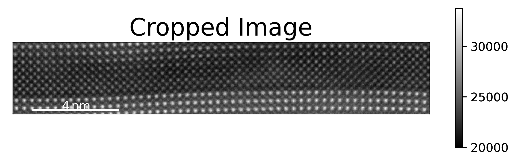
Open the PTO/SRO dataset

>>> image = hs.load('Cropped_PTO-SRO_Aligned.hspy')
>>> sampling = image.axes_manager[-1].scale #  nm/pix
>>> units = image.axes_manager[-1].units
>>> image.plot()

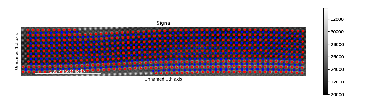
Open the pre-made PTO-SRO atom lattice.

>>> atom_lattice = am.load_atom_lattice_from_hdf5("Atom_Lattice_crop.hdf5")
>>> sublattice1 = atom_lattice.sublattice_list[0] #  Pb-Sr Sublattice
>>> sublattice2 = atom_lattice.sublattice_list[1] #  Ti-Ru Sublattice
>>> atom_lattice.plot()

Set up the Parameters

Plot the sublattice planes to see which zone_vector_index we use

>>> sublattice2.construct_zone_axes(atom_plane_tolerance=1)
>>> # sublattice2.plot_planes()

Set up parameters for calculate_atom_plane_curvature

>>> zone_vector_index = 0
>>> atom_planes = (2, 6) #  chooses the starting and ending atom planes
>>> vmin, vmax = 1, 2
>>> cmap = 'bwr' #  see matplotlib and colorcet for more colormaps
>>> title = 'Curvature Map'
>>> filename = None #  Set to a string if you want to save the map

Set the extra initial fitting parameters

>>> p0 = [14, 10, 24, 173]
>>> kwargs = {'p0': p0, 'maxfev': 1000}

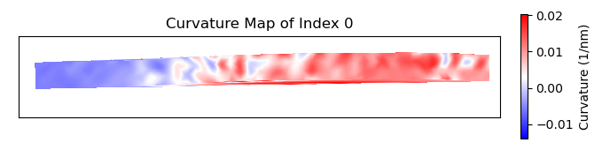
Calculate the Curvature of Atom Planes

We want to see the curvature in the SRO Sublattice

>>> curvature_map = tml.calculate_atom_plane_curvature(sublattice2, zone_vector_index,
...                     sampling=sampling, units=units, cmap=cmap, title=title,
...                     atom_planes=atom_planes, **kwargs)

When using plot_and_return_fits=True, the function will return the curve fittings, and plot each plane (plots not displayed).

>>> curvature_map, fittings = tml.calculate_atom_plane_curvature(sublattice2,
...                     zone_vector_index, sampling=sampling, units=units,
...                     cmap=cmap, title=title, atom_planes=atom_planes, **kwargs,
...                     plot_and_return_fits=True)