Interactive Image Filtering

The temul.signal_processing module allows one to filter images with a double Gaussian (band-pass) filter. Apart from the base functions, it can be done interactively with the temul.signal_processing.visualise_dg_filter() function. In this tutorial, we will see how to use the function on experimental data.

Load the Experimental Image

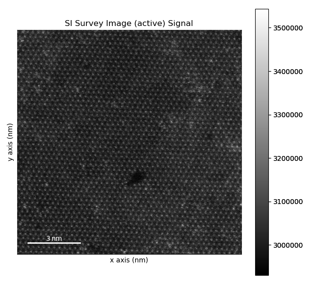
Here we load an example experimental atomic resolution image stored in the TEMUL package.

>>> import temul.api as tml
>>> from temul.example_data import load_Se_implanted_MoS2_data
>>> image = load_Se_implanted_MoS2_data()

Interactively Filter the Experimental Image

Run the temul.signal_processing.visualise_dg_filter() function. There are lots of other parameters too for customisation.

>>> tml.visualise_dg_filter(image)

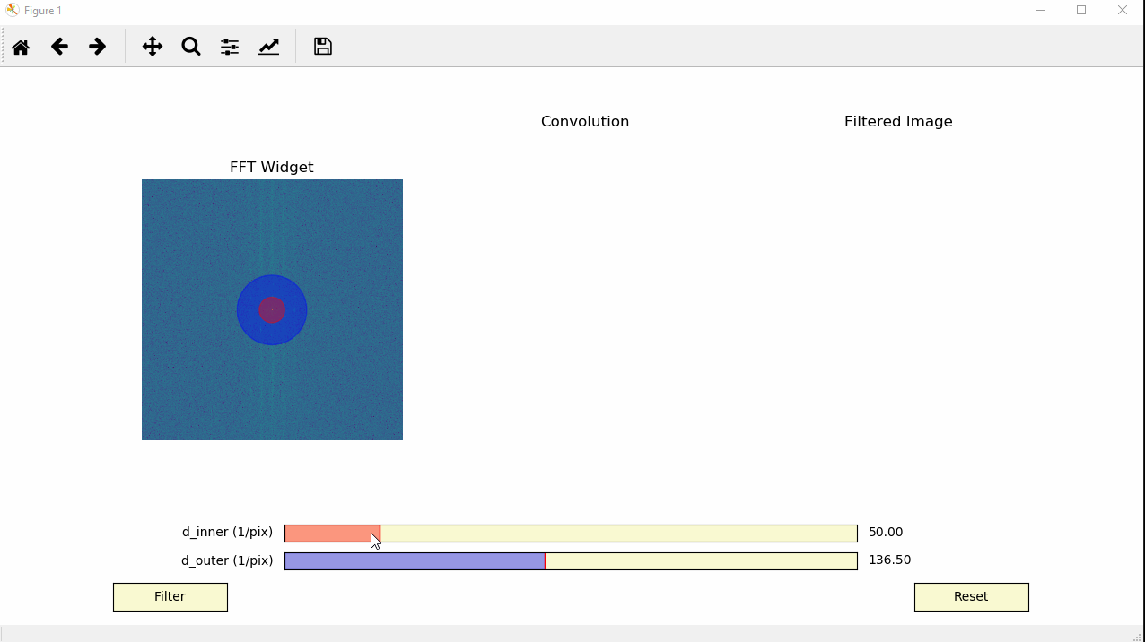
As we can see, an interactive window appears, showing the FFT (“FFT Widget”) of the image with the positions of the inner and outer Gaussian full width at half maximums (FWHMs). The inital FWHMs can be changed with the d_inner and d_outer parameters (limits can also be changed).

To change the two FWHMs interactively just use the sliders at the bottom of the window. Reset can be used to reset the FWHMs to their initial value, and Filter will display the “Convolution” of the FFT and double Gaussian filter as well as the inverse FFT (“Filtered Image”) of this convolution.

Return the Filtered Image

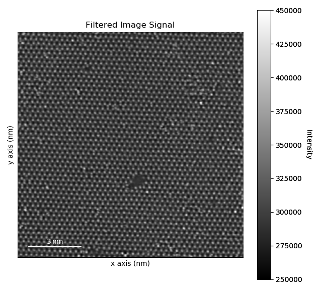
When we have suitable FWHMs for the inner and outer Gaussians, we can use the temul.signal_processing.double_gaussian_fft_filter() function the return a filtered image.

>>> filtered_image = tml.double_gaussian_fft_filter(image, 50, 150)
>>> image.plot()
>>> filtered_image.plot()

Details on the temul.signal_processing.double_gaussian_fft_filter_optimised() function can be found in the API documentation.